import pandas as pd
import numpy as np
import matplotlib.pyplot as plt
from sklearn.model_selection import train_test_split, GridSearchCV
from sklearn.tree import DecisionTreeClassifier
from sklearn import tree
from sklearn import datasets
from sklearn.preprocessing import StandardScaler

iris = datasets.load_iris()
iris.feature_names
# covariance:2개의 확률변수의 선형관계를 나타냄
# 선형성이 있으면 선형관계 알고리즘을 적용할수 있다 -> 그중에서 성능이 좋은 것을 선택
# 비선형인데 선형모델을 적용하면 좋은 결과를 얻을수 없다

# 공분산
# 데이터 단위(범위) 에 영향을 많이 받는 다  -> 상관계수를 사용
np.cov(iris.data[:, 0], iris.data[:, 1])
np.cov(iris.data[:, 2], iris.data[:, 3])

# 상관계수: -1 ~ 1 범위
# 공분산 / (A변수 표준편차 * B변수 표준편차)
np.corrcoef(iris.data[:, 0], iris.data[:, 3])

#sepal width, sepal length 선택
X = iris.data[:, [2, 3]]
y = iris.target
y.shape

# 표준화
# y 값을 표준화를 할 필요가 없기 때문에 데이터 분리 이후에 표준화를 하는 게 좋다
# parma_tree = {'criterion': ['gini', 'entropy'], 'max_depth' : np.arange(3,12)}

# 학습데이터 분리: 7:3, random_state 사용
X_train, X_test, y_train, y_test = \
    train_test_split(X, y, test_size=0.3,
                     random_state=123)

# 표준화 평균이 0 분산 1
sc =  StandardScaler()
X_train_sc = sc.fit_transform(X_train)
X_test_sc = sc.transform(X_test)

def dtree_grid_search(X, y, kfolds = 5):
  parma_tree = {'criterion': ['gini', 'entropy'], 'max_depth' : np.arange(3,12)}
  dtmodel = DecisionTreeClassifier()
  dt_gscv = GridSearchCV(dtmodel, parma_tree, cv = kfolds)
  dt_gscv.fit(X,y)
  return dt_gscv.best_params_

print(dtree_grid_search(X_train_sc, y_train, 5))

# tree모델 생성 및 학습: depth=3, entropy방식
# DecisionTreeClassifier 트리 분류
model = DecisionTreeClassifier(criterion='gini', max_depth=4)
model.fit(X_train_sc, y_train)

y_pred = model.predict(X_test_sc)
print('예측값:', y_pred)
print('실제값:', y_test)
더보기
{'criterion': 'gini', 'max_depth': 4}
예측값: [1 2 2 1 0 1 1 0 0 1 2 0 1 2 2 2 0 0 1 0 0 1 0 2 0 0 0 2 2 0 2 1 0 0 1 1 2
0 0 1 1 0 2 2 2]
실제값: [1 2 2 1 0 2 1 0 0 1 2 0 1 2 2 2 0 0 1 0 0 2 0 2 0 0 0 2 2 0 2 2 0 0 1 1 2
0 0 1 1 0 2 2 2]
from sklearn.metrics import accuracy_score

(y_test != y_pred).sum()
# accuracy_score 정확도
accuracy_score(y_test, y_pred)
# row, col 기준빈도수를 세어 도수분포표(frequency table)
# 2x2 배열 형태
con_mat = pd.crosstab(y_test, y_pred,
                      rownames=['예측치'],
                      colnames=['실제치'])
(con_mat[0][0]+con_mat[1][1]+con_mat[2][2])/len(y_test)
print(model.score(X_test_sc, y_test))
print(model.score(X_train_sc, y_train))

# 임의의 5개 데이터 쌍을 넣어서 예측
# 예측결과를 문자열로 출력
new_data = [[2.1, 3.2], [5.2, 7.8], [8.1, 3.2],
            [3.4, 6.3], [7.7, 4.5]]

# 표준화된 예측결과를 추가
new_pred = model.predict(sc.fit_transform(new_data)) # new_data 무조건 매트릭스형태
for i in new_pred:
    print(i, iris['target_names'][i])
더보기
0.9333333333333333
0.9809523809523809
0 setosa
1 versicolor
0 setosa
1 versicolor
2 virginica
from matplotlib.colors import ListedColormap
def plot_decision_region(X, y, classifier, test_idx=None,
                         resolution=0.02, title=''):
    markers = ('s', 'x', 'o', '^', 'v')
    colors = ('r', 'b', 'lightgreen', 'gray', 'cyan')
    cmap = ListedColormap(colors[:len(np.unique(y))])
    x1_min, x1_max = X[:,0].min()-1, X[:,0].max()+1
    print(x1_min, x1_max)
    x2_min, x2_max = X[:,1].min()-1, X[:,1].max()+1
    print(x2_min, x2_max)
    xx, yy = np.meshgrid(np.arange(x1_min, x1_max,
                                   resolution),
                         np.arange(x2_min, x2_max,
                                   resolution))
    # xx, yy를 평탄화 작업(1차원)으로 처리한후
    # 전치행렬로 변환
    Z = classifier.predict(np.array([xx.ravel(),
                                     yy.ravel()]).T)
    Z = Z.reshape(xx.shape)

    plt.contourf(xx, yy, Z, alpha=0.5, cmap=cmap)
    plt.xlim(xx.min(), xx.max())
    plt.ylim(yy.min(), yy.max())

    X_test = X[test_idx, :]
    for idx, cl in enumerate(np.unique(y)):
        plt.scatter(x=X[y==cl, 0], y=X[y==cl, 1],
                    c=cmap(idx), marker=markers[idx],
                    label=cl)
    if test_idx:
        X_test = X[test_idx, :]
        plt.scatter(X_test[:, 0], X_test[:, 1], c=[],
                    linewidth=1, marker='o',
                    label='TestData')
    plt.xlabel('꽃잎(petal) 길이')
    plt.ylabel('꽃잎(petal) 너비')
    plt.legend(loc=2)
    plt.title=title
    plt.show()
x_combined_std = np.vstack((X_train_sc, X_test_sc))
y_combined = np.hstack((y_train, y_test))
plot_decision_region(X=x_combined_std, y=y_combined,
classifier=model,
test_idx=range(105, 150),
title='Decision Tree')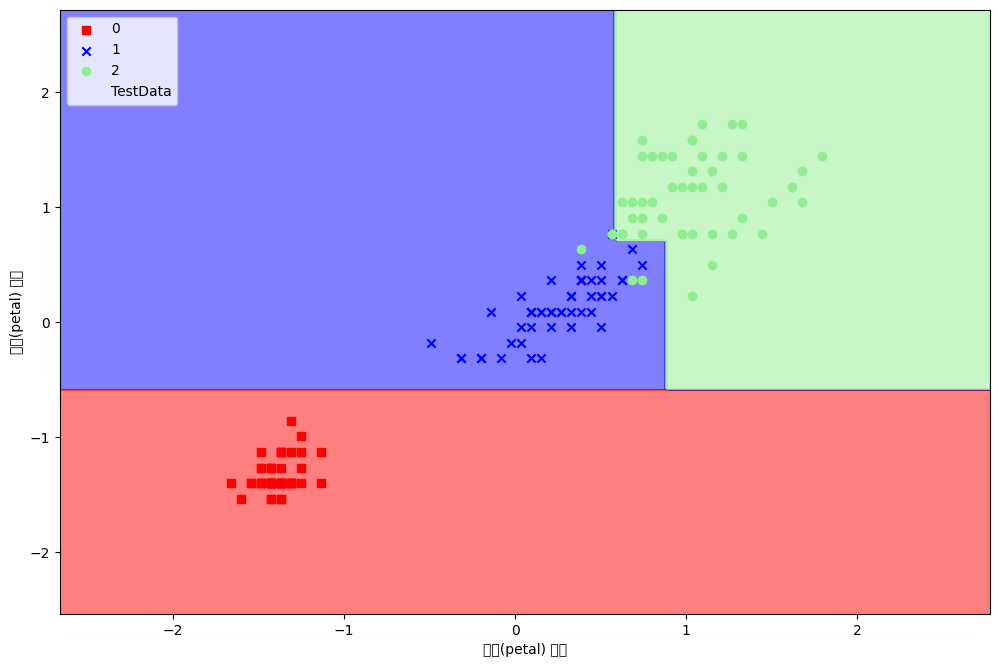
from io import StringIO
import pydotplus

dot_data = StringIO()
tree.export_graphviz(model, out_file=dot_data,
                     feature_names=iris.feature_names[2:4],
                     class_names=iris.target_names)
graph = pydotplus.graph_from_dot_data(dot_data.getvalue())
graph.write_png('tree2.png')
img = plt.imread('tree2.png')
plt.rcParams.update({'figure.dpi':'100',
                     'figure.figsize':[12,8]})
plt.imshow(img)
plt.show()

# 엔트로피 entropy 가 0.0일 경우 리프 노드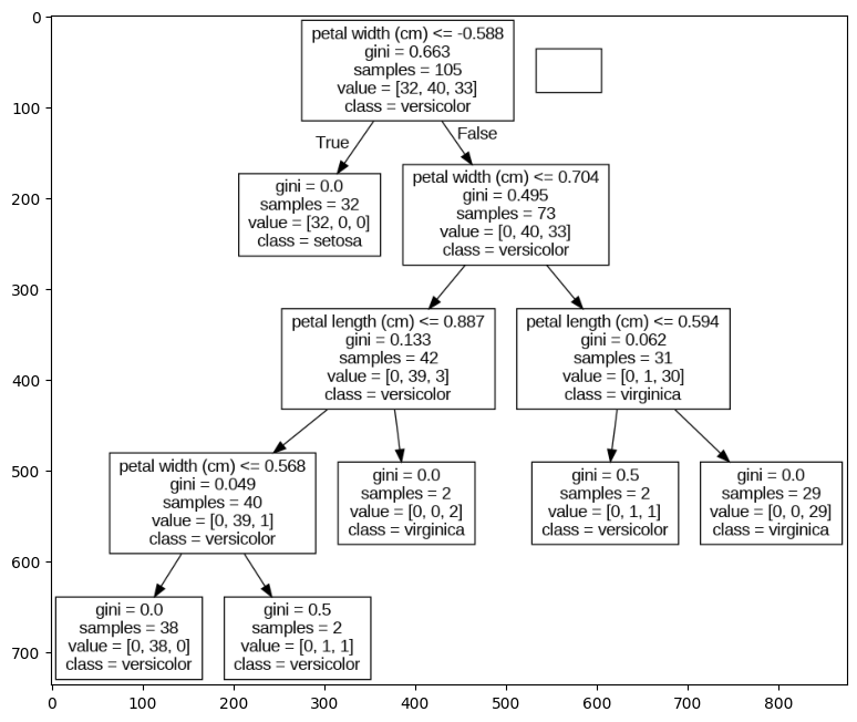
'Colab > 머신러닝' 카테고리의 다른 글
| 10. 랜덤 포레스트 (random forest) 02 (0) | 2023.03.09 |
|---|---|
| 09. 랜덤 포레스트 (random forest) 01 (0) | 2023.03.09 |
| 07. 결정 트리 (Decision Tree) 01 (0) | 2023.03.08 |
| 06. K-최근접 이웃 회귀 K-NN Regression (0) | 2023.03.06 |
| 05. 로지스틱 회귀분석 Logistic Regression (0) | 2023.03.03 |