import numpy as np
import pandas as pd
import matplotlib.pyplot as plt
from  sklearn.datasets import make_blobs, load_iris
from sklearn.cluster import KMeans
from sklearn.metrics import silhouette_score

plt.rc('font', family='NanumBarunGothic')
iris = load_iris()
# print(iris)
X = iris.data
y = iris.target
# 시각화를 위해 컬럼을 합친다
df = pd.DataFrame(data=X, columns=iris.feature_names)
df['target'] = y
# df.loc[:, 'target']=pd.Dataframe(y)# inertia : 군집내의 데이터 거리 제곱의 함
ks = range(1,10)
inertias=[]
for k in ks:
model = KMeans(n_clusters=k, n_init='auto')
model.fit(X)
inertias.append(model.inertia_)
print(inertias)
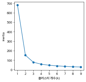
# 완만하게 떨어지는 시점
plt.figure(figsize=(4,4))
plt.plot(ks, inertias,'-o')
plt.xlabel('클러스터 개수(k)')
plt.ylabel('inertia')
plt.xticks(ks)
plt.show()
# 3에서 기울기가 완만해지고 있다
# 응집도가 3이 가장높다고 볼수있다더보기
[681.3706, 152.3479517603579, 78.85566582597731, 57.22847321428572, 46.71230193050193, 39.620375014280896, 34.640499346191575, 30.1865551948052, 28.345888395230503]
model = KMeans(n_clusters=4, n_init = 'auto', max_iter=500, random_state=123, algorithm='lloyd', verbose=2)
model.fit(X)
centers = model.cluster_centers_ # 각각의 군집의 중심점(centeroid)
y_pred = model.predict(X)
y_pred
더보기
Initialization complete
Iteration 0, inertia 110.44999999999999.
Iteration 1, inertia 64.9957017106938.
Iteration 2, inertia 62.95179896990007.
Iteration 3, inertia 61.70309548611112.
Iteration 4, inertia 60.79023611394881.
Iteration 5, inertia 60.23232602544927.
Iteration 6, inertia 59.54050318848107.
Iteration 7, inertia 59.14898931572629.
Iteration 8, inertia 58.90258285274895.
Iteration 9, inertia 58.36929541700745.
Iteration 10, inertia 58.100180684210855.
Iteration 11, inertia 57.619232126506375.
Iteration 12, inertia 57.53024031422781.
Iteration 13, inertia 57.38387326549494.
Converged at iteration 13: strict convergence.
array([1, 1, 1, 1, 1, 1, 1, 1, 1, 1, 1, 1, 1, 1, 1, 1, 1, 1, 1, 1, 1, 1,
       1, 1, 1, 1, 1, 1, 1, 1, 1, 1, 1, 1, 1, 1, 1, 1, 1, 1, 1, 1, 1, 1,
       1, 1, 1, 1, 1, 1, 3, 3, 3, 2, 3, 2, 3, 2, 3, 2, 2, 2, 2, 3, 2, 3,
       2, 2, 3, 2, 3, 2, 3, 3, 3, 3, 3, 3, 3, 2, 2, 2, 2, 3, 2, 3, 3, 2,
       2, 2, 2, 3, 2, 2, 2, 2, 2, 2, 2, 2, 0, 3, 0, 3, 0, 0, 2, 0, 0, 0,
       3, 3, 0, 3, 3, 3, 3, 0, 0, 3, 0, 3, 0, 3, 0, 0, 3, 3, 3, 0, 0, 0,
       3, 3, 3, 0, 0, 3, 3, 0, 0, 3, 3, 0, 0, 3, 3, 3, 3, 3], dtype=int32)
# 시각화를 위해 DataFrame화
clust_df = df.copy()
clust_df['clust']= y_pred
print(silhouette_score(X,y_pred))더보기
0.49535632852884987
import seaborn as sns

plt.figure(figsize=(20,6))
plt.subplot(131)
sns.scatterplot(x=clust_df.iloc[:,0],
                y=clust_df.iloc[:,1],
                data=clust_df, hue=model.labels_,
                palette='coolwarm')
plt.scatter(centers[:,0],centers[:,1],c='green', alpha=0.9, s=30)

# ---------------------------------------------------------------
plt.subplot(132)
sns.scatterplot(x=clust_df.iloc[:,0],
                y=clust_df.iloc[:,2],
                data=clust_df, hue=model.labels_,
                palette='coolwarm')
plt.scatter(centers[:,0],centers[:,2],c='green', alpha=0.9, s=30)

# ---------------------------------------------------------------
plt.subplot(133)
sns.scatterplot(x=clust_df.iloc[:,0],
                y=clust_df.iloc[:,3],
                data=clust_df, hue=model.labels_,
                palette='coolwarm')
plt.scatter(centers[:,0],centers[:,3],c='green', alpha=0.9, s=30)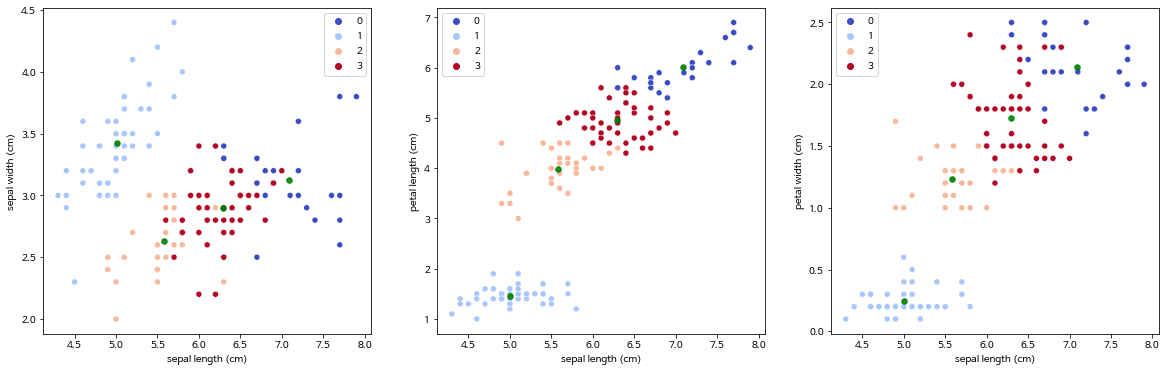
from matplotlib import projections
# 3차원 시각화
fig = plt.figure(figsize=(8,8))
ax = fig.add_subplot(111, projection='3d')
# data
ax.scatter(clust_df.iloc[:,0],clust_df.iloc[:,1],clust_df.iloc[:,2],c=clust_df.clust, s=10, cmap='rainbow', alpha=1)
# centeroid
ax.scatter(centers[:,0],centers[:,1],centers[:,2], c='black', s=100, marker='*')
plt.show()
'Colab > 머신러닝' 카테고리의 다른 글
| 16. K-평균 (K-means) & 실루엣 계수 (silhouette coefficient) 01 (0) | 2023.03.10 |
|---|---|
| 15. XGBoost 01 (0) | 2023.03.10 |
| 14. GBoost 02 (0) | 2023.03.10 |
| 13. GBoost 01 (0) | 2023.03.10 |
| 12. 부스팅(Boosting) 01 (0) | 2023.03.09 |